Connecting an Analog Oscilloscope with Edge IO and Node-RED

Connecting an Analog Oscilloscope with Edge IO and Node-RED

Learn how to use the analog oscilloscope Node-RED flow with your Edge IO

This article covers the workflow to view analog sensor data from the Edge IO locally in Node-RED. It will utilize a Tulip Node-RED library flow that can be imported on your Edge IO.

By the end of this article, you will have the following flow within Node-RED and be able to view a live, local visualization of the device data.

You will complete the following steps:

1. Hardware Setup: Wire the Edge IO
2. Node-RED Setup: Import, edit, and deploy a Node-RED flow from the Tulip Library

What you will need is:

• An Edge IO registered to your Tulip account

• Sensors to connect to the various Edge IO analog ports, such as:

  • Current transformer (for the Differential ADC)
  • Pressure Sensor (for the 0-10V SAR ADC)
  • IEPE Vibration Sensor (for the Current-Source ADC)

Note: In this flow, the analog data is not persisted or sent to Tulip. The flow is primarily intended to be a diagnostic tool during development to visualize the current data being captured by the analog sensors.

1. Hardware Setup - Wire the Edge IO

The exact sensors that you wire to the Edge IO are up to you. This flow is sensor agnostic and outputs the voltage measured at the analog input to the Edge IO. However, an example set of sensors that you could wire include:

• Differential ADC: A current transformer
• SAR ADC: A pressure sensor or other sensor that outputs 0-10V (and optionally is powered by 24V)
• Current-Source ADC: An IEPE vibration sensor

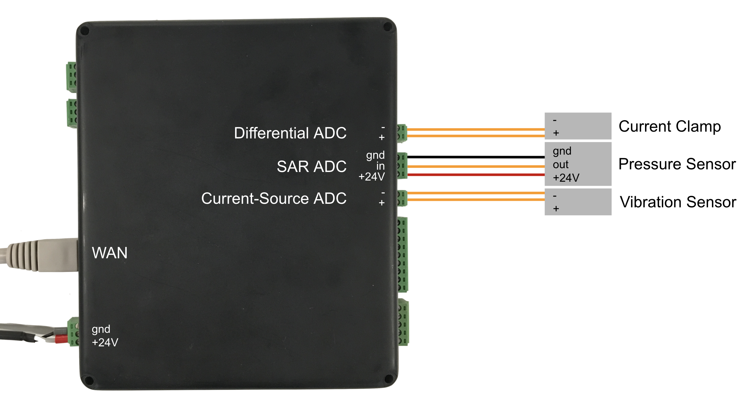
Additionally, ensure that you’ve powered the device and connected the device to your network by plugging an ethernet cable into the WAN port or via wi-fi.

2. Node-RED Setup

Open the Device Portal on the Edge IO. Launch the Node-RED Editor using the following credentials:

• Username: admin
• Password: Your Edge IO password

See more information here to get started with Node-RED on Edge IO.

2a. Import Library Flow

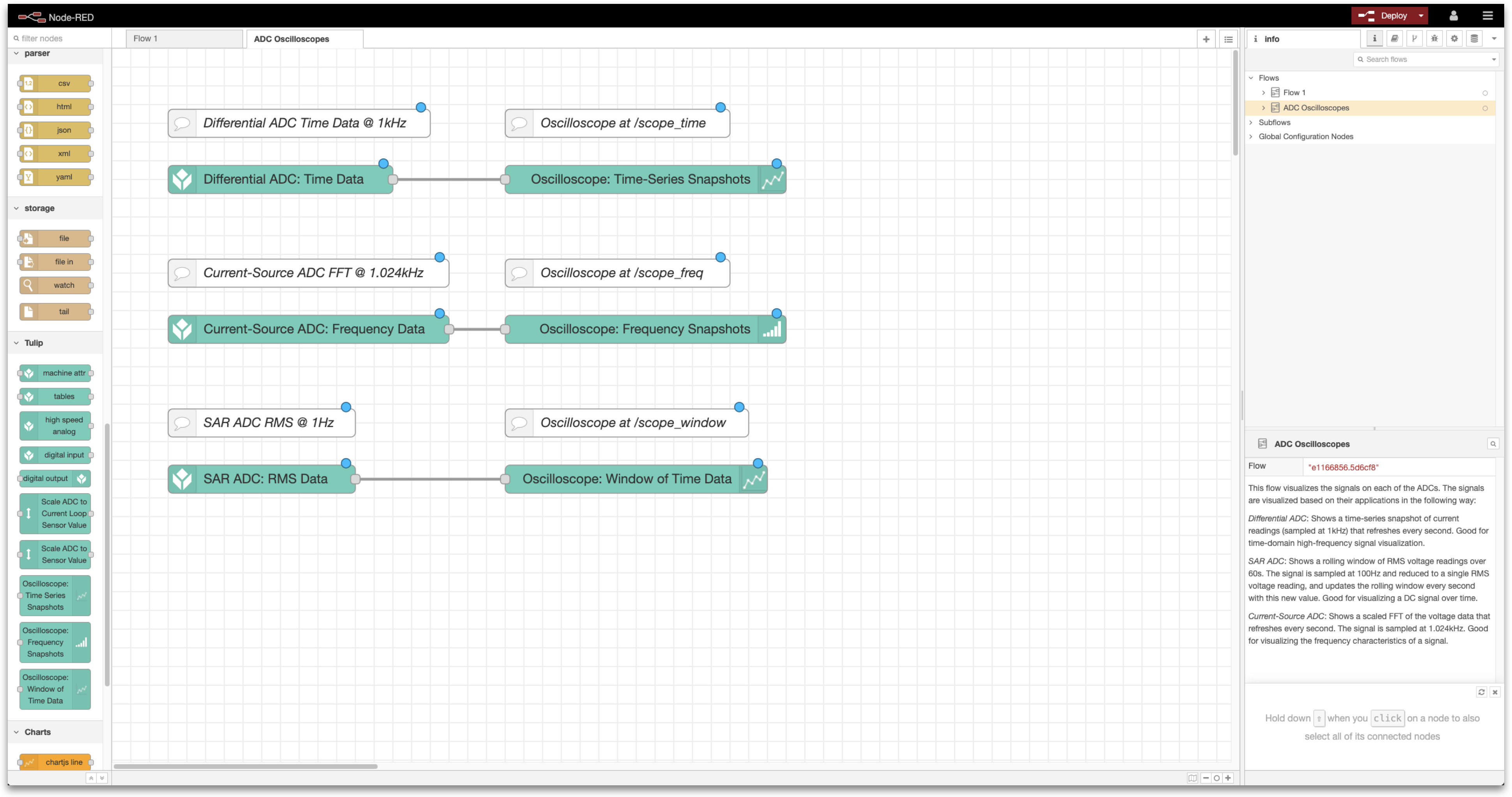
To import the library flow, follow the steps in our Importing Tulip Node-RED Flows document. The flow to import is analog_oscilloscopes.json and importing creates the ADC Oscilloscopes tab in the editor.

2b. Overview of the Flow

This flow is comprised of three separate workstreams to visualize signals on each of the ADCs:

Differential ADC

Generates a time-series snapshot of current readings that refresh every second. This can be used to visualize time-domain high-frequency signals.

This flow is comprised of two functional nodes:

1. Differential ADC: Time Data

   • Purpose: Samples the differential ADC at 1 kHz, with 1000-sample buffers. Outputs the data in each buffer. By default, this will output continuously once per second.

2. Oscilloscope: Time-Series Snapshots

   • Purpose: Configure subflow to generate a visualization of a buffer of time data, which is accessible at :1880/scope_time.

Current-Source ADC

Generates a scaled FFT of the voltage data that refreshes every second. This can be used to visualize the frequency characteristics of a signal.

This flow is comprised of two functional nodes:

1. Current-Source ADC: Frequency Data

   • Purpose: Samples the current-source ADC at 1.024kHz with 1024-sample buffers. Outputs the FFT of each buffer. By default, this will output continuously once per second.

2. Oscilloscope: Frequency Snapshots

   • Purpose: Configure subflow to generate a visualization of an FFT, which is accessible at :1880/scope_freq.

SAR ADC

Generates a rolling window of RMS voltage readings over 60 seconds. This can be used to visualize a DC signal over time.

This flow is comprised of two functional nodes:

1. SAR ADC: RMS Data

   • Purpose: Samples the SAR ADC at 100Hz with 100-sample buffers. Outputs the RMS value of each buffer. By default, this will output continuously.

2. Oscilloscope: Window of Time Data

   • Purpose: Configure subflow to generate a visualization of a rolling window of data, which is accessible at :1880/scope_window.

2c. Deploy the Flow

With the Node-RED flow imported, you can Deploy your flow from the top right and begin to see the data from the Edge IO analog inputs.

2d. Edit the Flow

Many details of this flow can be edited depending on the sensors you use and the values that they output. Examples of edits that you can make include:

• Displaying measured sensor inputs instead of voltage into ADC.

  • For example, let’s say you’ve connected to the Differential ADC a CR3111-3000 current transformer, which has a turns ratio of 3000 (and will output 1mA when measuring 3A)
  • Edit the Oscilloscope: Time-Series Snapshots node to have a Sensor Scale of 3000, a Y-Axis Labelof “Measured Current (A)”, and Min Y Value and Max Y Value that match the expected min and max expected measured currents

• View a different type of data for given analog input.

  • For example, if you’d like to view the time-series data for the current-source ADC (instead of the FFT), then you can select the Current-Source ADC: Frequency Data node and edit its configuration node to add Time-domain data as an output and enable Time data as an output.

• Alter the parameters of the rolling window of time data

  • If you want to visualize the data from the SAR ADC over a longer (or shorter) period of time, you can edit the Window Length of the Oscilloscope: Window of Time Data node.
  • The window resolution should match the time of a buffer; if you have 100-sample buffers captured at 200Hz, then your buffers are 0.5 seconds long and the window resolution should be updated to 0.5 seconds.

3. Flow Visualizations

By navigating to the following paths, you’ll be able to visualize the data for the analog inputs. Below we include graphs both for when the input is “floating” (i.e. when there is no sensor plugged in), and an example graph from when the suggested sensor from the Hardware Setup is plugged in

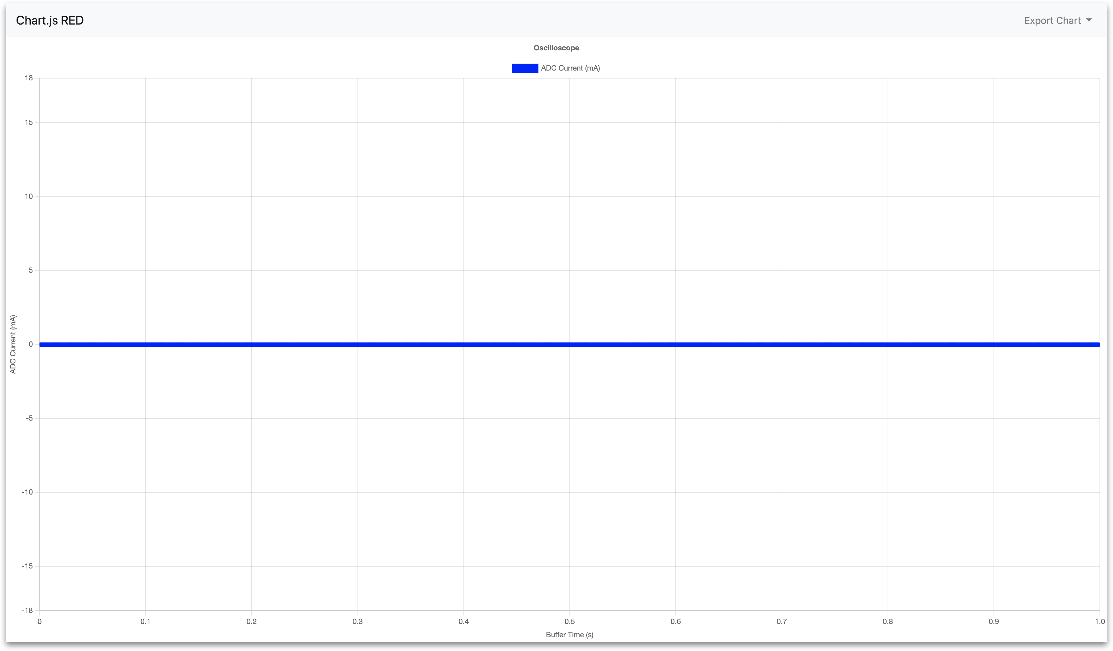
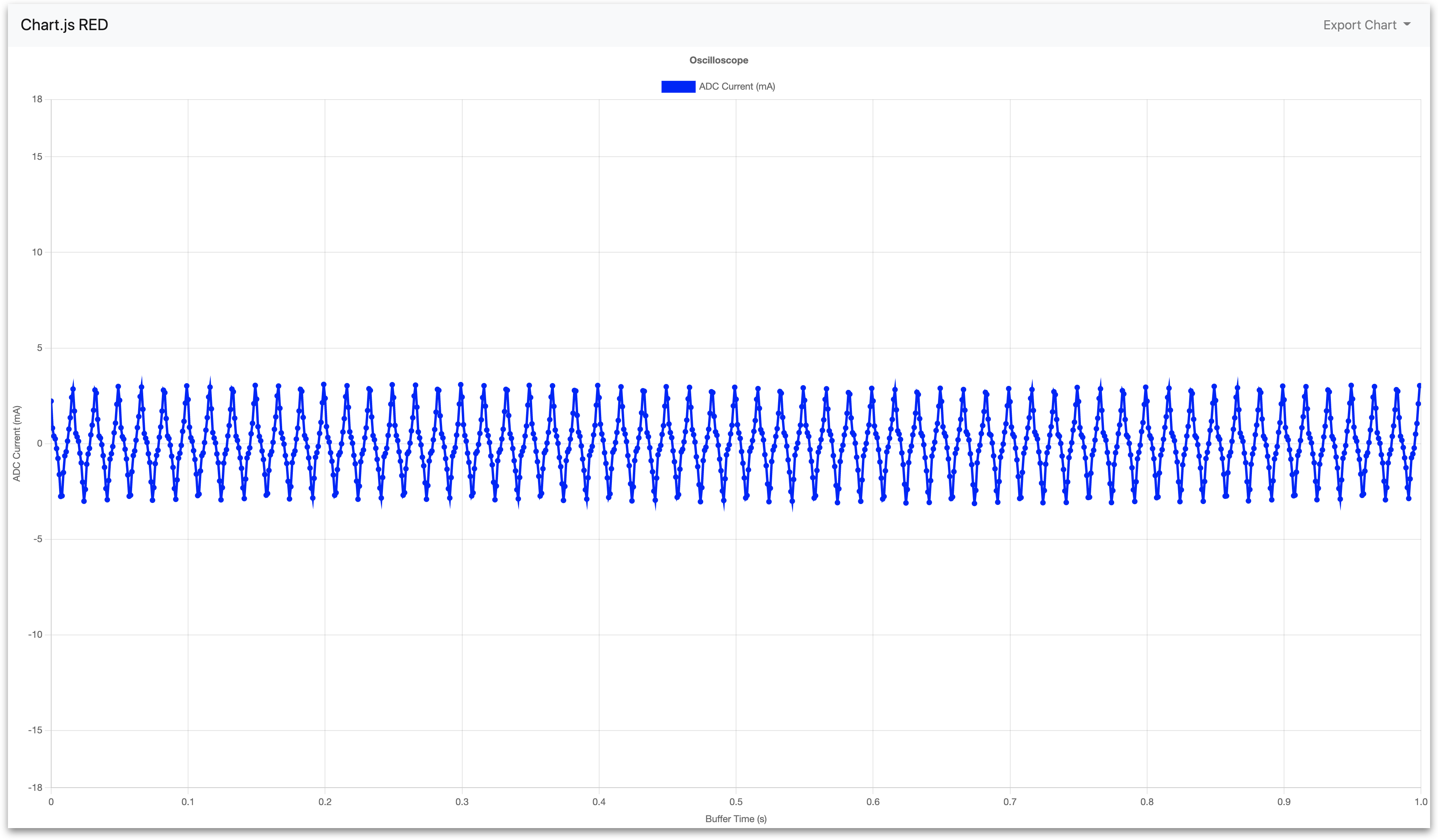
3a. Differential ADC

• :1880/scope_time

No sensor connected to Differential ADC:

Current transformer connected to Differential ADC:

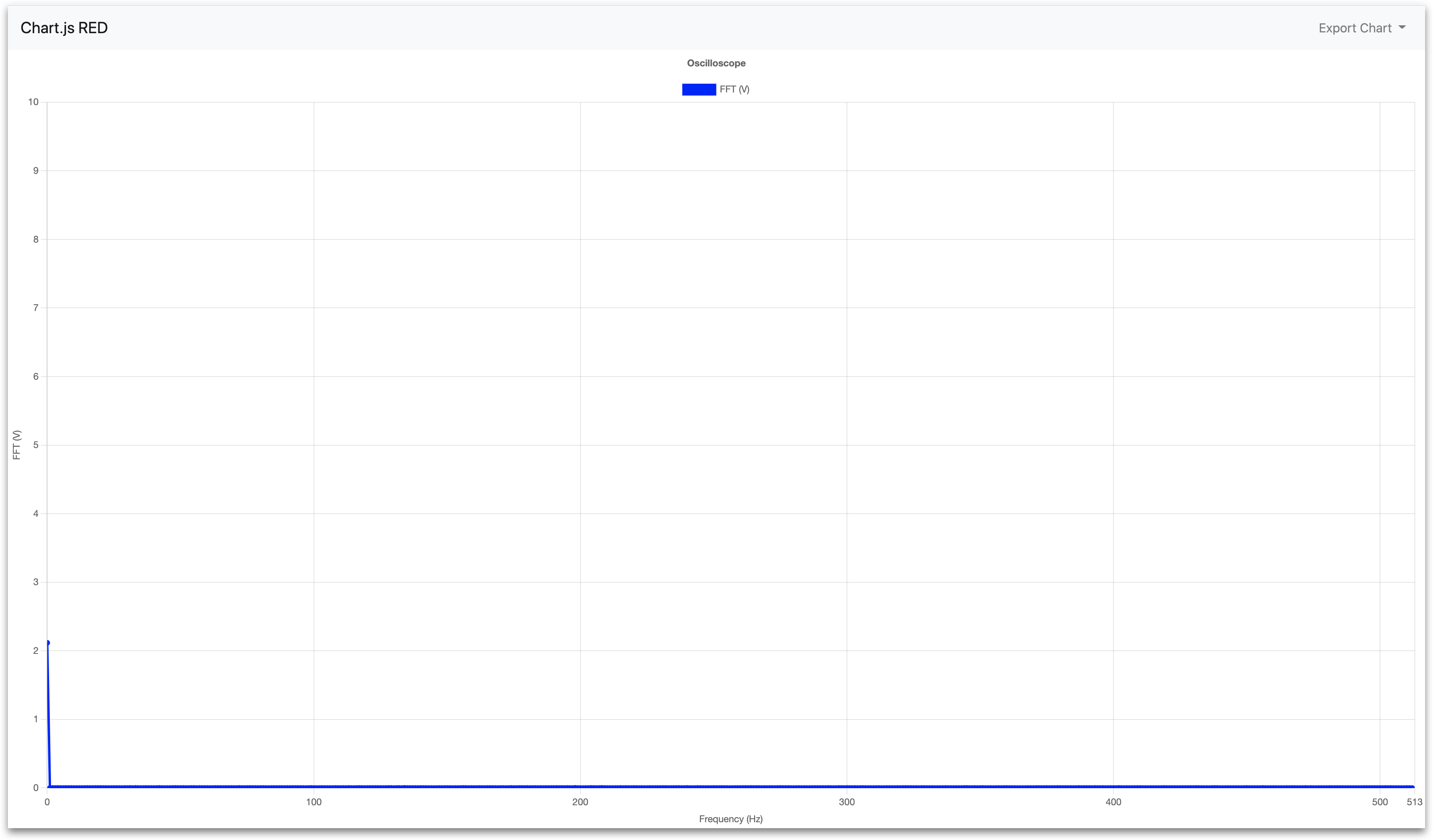
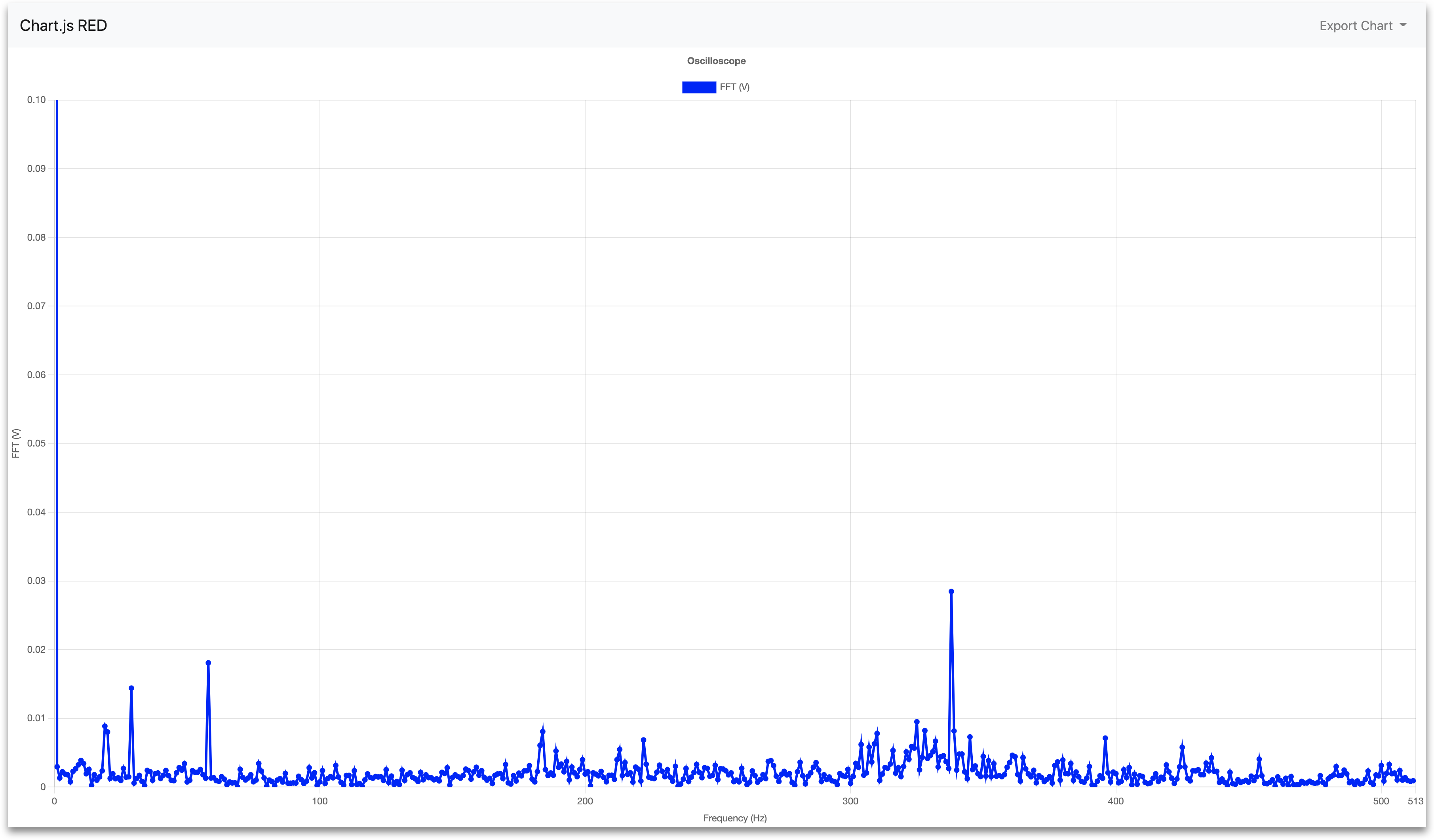
3b. Current-Source ADC

• :1880/scope_freq

No sensor connected to Current-Source ADC:

Vibration sensor connected to Current-Source ADC (with adjusted Y-Axis scale for better resolution):

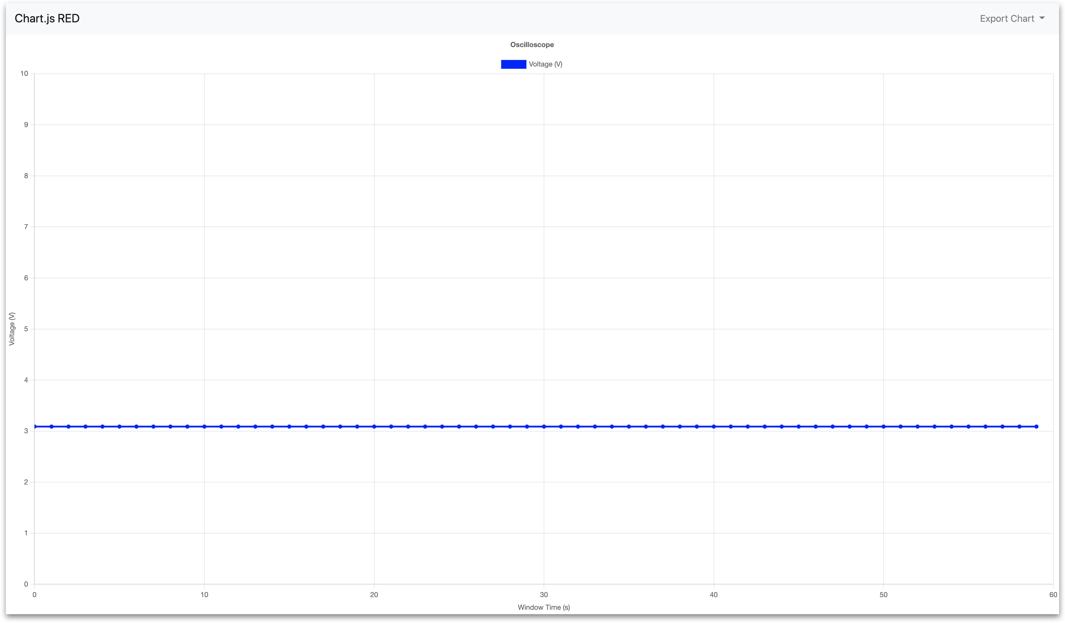
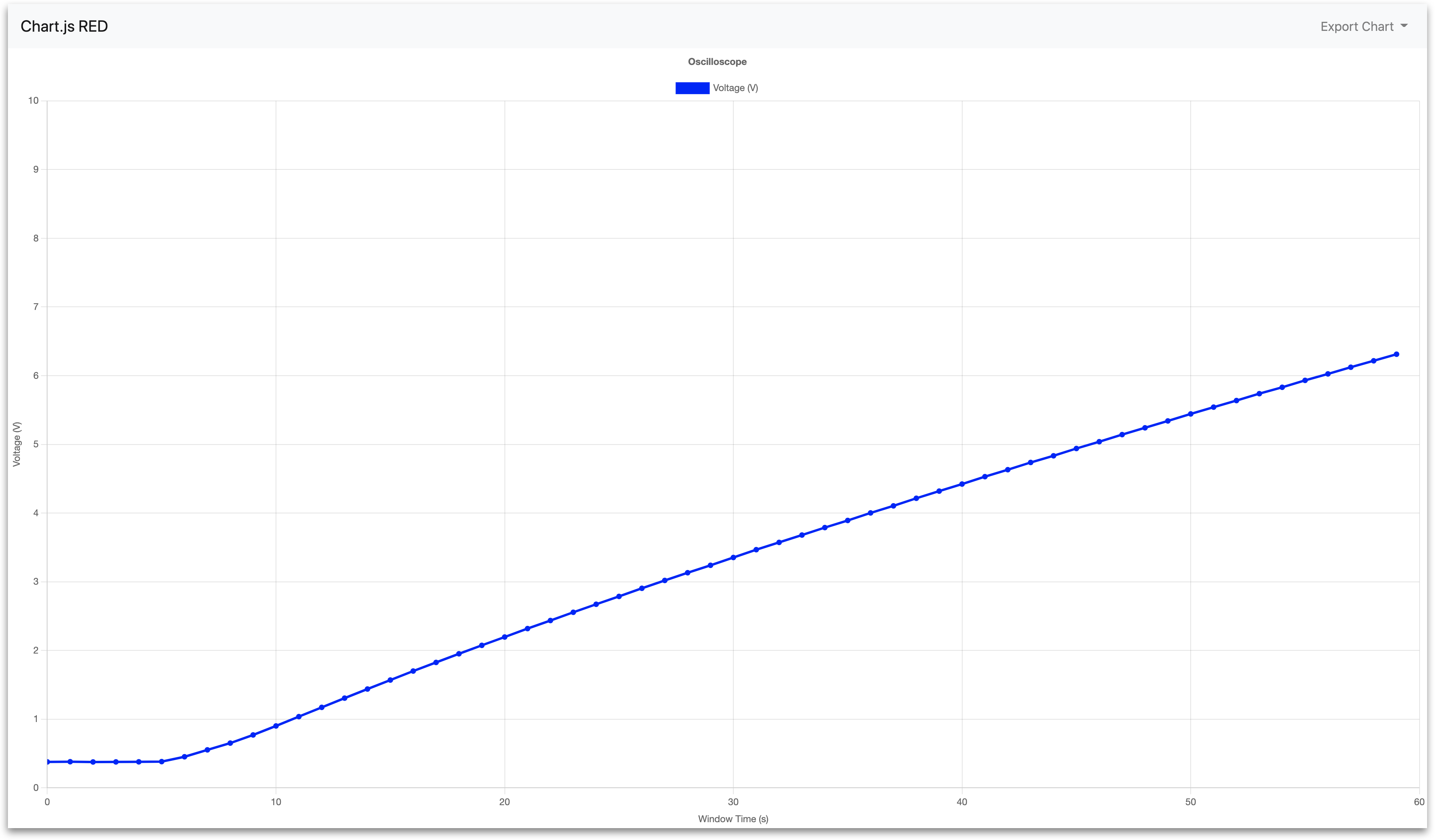
3c. SAR ADC

• :1880/scope_window

No sensor connected to SAR ADC:

Pressure sensor connected to Current-Source ADC:

Technical Details of the Node-RED Flow

Below is a detailed summary of the nodes and their default configuration parameters imported with the analog_oscilloscopes.json file.

Differential ADC

1. Differential ADC: Time Data

   • Purpose: Samples the differential ADC at 1 kHz, with 1000-sample buffers. By default, this will output continuously.

   • Node type: High-speed-analog

   • Default properties:

     • Analog Config - Differential ADC RMS @ 1kHZ

       • Select ADC to Configure - Differential ADC
       • Enabled Outputs - RMS
       • Buffer Size - 1000
       • Sampling Frequency (Hz) - 1000

     • Data Type - Time

     • Output Mode - Continuous

     • Refresh Rate (seconds) - 1

2. Oscilloscope: Time-Series Snapshots

   • Purpose: Configure subflow to generate visualization, which is accessible at :1880/scope_time.

   • Node type: Subflow

   • Default properties:

     • Chart Name - scope_time
     • Min Y Value - -18
     • Max Y Value - 18
     • Y Axis Label - ADC Current (mA)
     • Sensor Scale - 1000
     • Sensor Offset - 0

Current-Source ADC

1. Current-Source ADC: Frequency Data

   • Purpose: Samples the current-source ADC at 1.024kHz with 1024-sample buffers. By default, this will output continuously.

   • Node type: High-speed-analog

   • Default properties:

     • Analog Config - Current-Source ADC @ 1kHz

       • Select ADC to Configure - Current-Source ADC
       • Enabled Outputs - Frequency-Domain (FFT)
       • Buffer Size - 1024
       • Sampling Frequency (Hz) - 1024

     • Data Type - Frequency (FFT)

     • Output Mode - Continuous

     • Refresh Rate (seconds) - 1

2. Oscilloscope: Frequency Snapshots

   • Purpose: Configure subflow to generate visualization, which is accessible at :1880/scope_freq.

   • Node type: Subflow

   • Default properties:

     • Chart Name - scope_freq
     • Max Y Value - 10
     • Y Axis Label - FFT (V)
     • Sensor Scale - 1
     • X Axis Type - Linear
     • Y Axis Type - Linear

SAR ADC

1. SAR ADC: RMS Data

   • Purpose: Samples the SAR ADC at 100Hz with 100-sample buffers. By default, this will output continuously.

   • Node type: High-speed-analog

   • Default properties:

     • Analog Config - SAR ADC: RMS @ 100HZ

       • Select ADC to Configure - SAR ADC
       • Enabled Outputs - RMS
       • Buffer Size - 100
       • Sampling Frequency (Hz) - 100

     • Data Type - RMS

     • Output Mode - Continuous

     • Refresh Rate (seconds) - 1

2. Oscilloscope: Window of Time Data

   • Purpose: Configure subflow to generate visualization, which is accessible at :1880/scope_window.

   • Node type: Subflow

   • Default properties:

     • Chart Name - scope_window
     • Min Y Value - 0
     • Max Y Value - 10
     • Y Axis Label - Voltage (V)
     • Sensor Scale - 1
     • Sensor Offset - 0
     • Window Length (samples) - 60
     • Window Resolution (s) - 1

Further Reading

• Node-RED's documentation
• Connecting a 4-20 mA Sensor with Edge IO and Node-RED
• Managing Machine States and Part Counts with Edge IO and Node-RED

Did you find what you were looking for?

You can also head to community.tulip.co to post your question or see if others have faced a similar question!